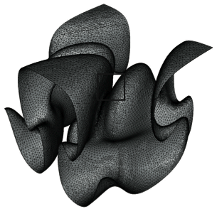
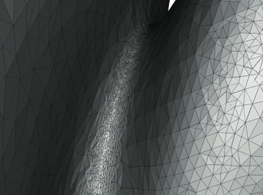
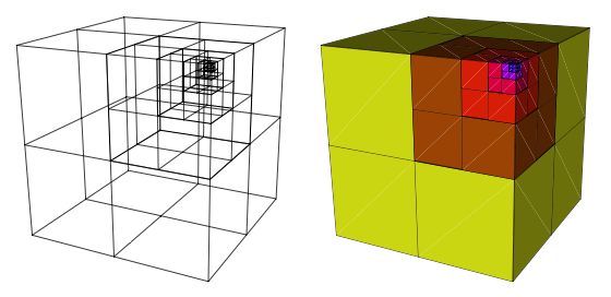
DOUAR is a new finite element code for the solution of the Stokes and energy (or heat transport) equations that has been purposely designed to address crustal- scale to mantle-scale flow problems in three dimensions. Although it is based on an Eulerian description of deformation and flow, the code has the ability to track interfaces and, in particular, the free surface, by using a dual representation based on a set of particles placed on the interface and the computation of a level set function on the nodes of the finite element grid, thus ensuring accuracy and efficiency. The code makes also use of a new method to compute the dynamic Delaunay triangulation connecting the particles based on a non-Euclidian, curvilinear metrics, ensuring that the density of particles remains uniform and/or dynamically adapted to the curvature of the interface. On the following figures are shown the geometry and triangulation of an originally flat surface deformed by a prescribed periodic and incompressible velocity field. The right panel is a close-up of a region (indicated on the left panel) where the surface curvature has become very large.
The finite element discretization is based on a non-uniform, yet regular octree division of space within a unit cube that allows to adapt the finite element discretization at will, i.e. in regions of strong velocity gradient or high interface curvature, with efficiency. On the following figure is shown the example of a simple octree discretization of the unit cube. The unit cube is divided in 8 sub-cubes, which can be arbitrarily divided into 8 sub-sub-cubes, and so on. The sub-cubes that remain undivided at the end of the construction of the octree are called leaves which are used here as finite elements with which the partial differential equations are solved.
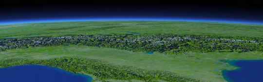
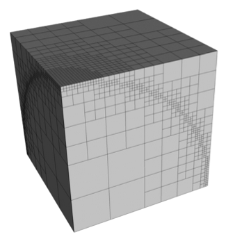
On this next figure is shown an octree designed to represent a spherical shell of unit radius. It has been constructed so that the region surrounding the shell is discretized with leaves of level 6. It has also been smoothened, i.e. the condition that no two adjacent leaves (or elements) can vary in size by more than one level of octree division has been applied.
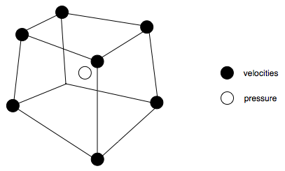
The finite elements are cubes (the leaves of the octree) in which a q1-p0 interpolation scheme is used:
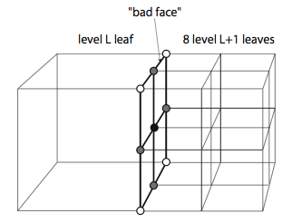
Nodal incompatibilities across faces separating elements of differing size are dealt with by introducing linear constraints among nodal degrees of freedom. The interface between two sets of leaves of different level is called a badface. These bad faces contain nodes that belong to the smaller elements on one side of the face and not to the larger element on the other side of the face. These nodes are colored in black and grey on the figure. Using the finite element method, one can only solve for velocity components and temperature on nodes that belong to elements on both sides of the face(the white nodes). To obtain values at the incompatible nodes, one needs to impose additional linear constraints that constrain the solution at the grey mid-side nodes to be the mean of the two adjacent white nodes, and the solution at the central black node to be the mean of the four corners nodes.
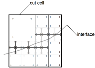
Discontinuities in material properties across the interfaces is accommodated by the use of a novel method (which we called divFEM) to integrate the finite element equations in which the elemental volume is divided by a local octree to an appropriate depth (resolution). From the values of the level set functions, the position of each element with respect to each interface is known as well as possible intersections between the element and the interfaces. This information is used to determine the material making up the element, assuming that interfaces are material boundaries. When an element is intersected by one or several interfaces, the value of the level set functions at the nodes of the elements are used to compute the part or volume of the element that is in each of the materials. These volumes are used to perform the volume integration of the finite element equations To determine the volume that is on the positive side of the interface cutting a given element (the cut cell), an octree division of cut cells is performed down to level l. The level set function is interpolated to the internal nodes and used to determine which part of the volume (positive or negative) each sub-cell belongs to. The relative positive volumes in the remaining cut cells are estimated using an approximate formula. In those cut cells, material properties are averaged if possible, otherwise the property corresponding to material representing the largest volume in the cut cell is used. On the following figure is shown the subdivision of an element cut by a surface, and the gauss quadrature integration points ('+' signs).
A variety of rheologies have been implemented including linear, non-linear and thermally activated creep and brittle (or plastic) frictional deformation. A simple smoothing operator has been defined to avoid checkerboard oscillations in pressure that tend to develop when using a highly irregular octree discretization and the tri-linear (or q1-p0 ) finite element.
A three-dimensional cloud of particles is used to track material properties that depend on the integrated history of deformation (the integrated strain, for example); its density is variable and dynamically adapted to the computed flow.
The large system of algebraic equations that results from the finite element discretization and linearization of the basic partial differential equations is solved using a multi-frontal massively parallel direct solver that can efficiently factorize poorly conditioned systems resulting from the highly non-linear rheolgy and the presence of the free surface. The code is almost entirely parallelized.
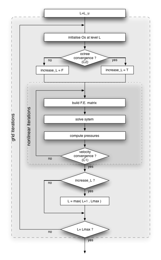
Schematically, the code structure is built upon three imbricated loops, as sketched on the following figure: the outer loop (not shown) is the time stepping, the second one is the progressive adaptive grid construction, and the inner third one is the nonlinear iterations one.
In order to illustrate how the octree refinement algorithm concretely works, to justify its implementation in DOUAR and to demonstrate its efficiency, we have carried out numerical experiments of two-dimensional and three-dimensional punches indenting a rigid, perfectly plastic von Mises half-space. The analytical solution to the two-dimensional problem is to be found in many textbooks (Hill, 1950)(Kachanov, 2004), or (Freudenthal and Geiringer, 1958) for a more mathematical approach.
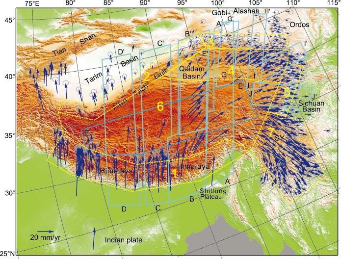
Moreover, since the late 70's, a simple analogy has been made between the tectonics of Asia and the deformation of a rigidly indented rigid-plastic solid: India is analogous to the indenter and the great strike-slip faults, such as the Kunlun Fault System, correspond to slip lines (Molnar and Tapponier, 1975). This analogy has been the subject of physical (Davy and Cobbold, 1988) and numerical modelling (Houseman and England, 1993, among many others) and has given rise to an abundant litterature. More recently, GPS data seem to indicate that the velocity measurements fit to a certain degree an indenter type of velocity field (Zhang et al., 2004) :
In the two-dimensional case, the analytical solution is known, and the slip-line solution is shown on the following figure:
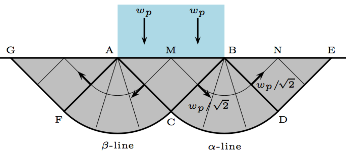
The slip lines consist of a curvilinear mesh of two families of lines, which always cross each other at right angles. The velocity distribution and stress state can be determined from the geometry of these lines. An undeformed wedge of material forms an active so-called Rankine zone below the punch with angles π/4. This wedge pushes material outwards, causing passive Rankine zones to form with angles π/4. The transition zones are circular. In order to carry out two-dimensional simulations, we have set no-slip boundary conditions on the walls of the cube so that no flux of material is allowed outside the unit cube, and we have imposed a velocity v = (0, 0, -wp) for nodes whose coordinates (x, y, z ) verify 0≤x≤1, -Δy/2 ≤ y ≤ +Δy/2 and z = 1. In fact, this corresponds to replicating the 2D punch problem (plane Oxy) in the third dimension (along Oz ).
The (dimensionless) parameters used to run the simulations are: gravity g = 0, punch width Δy = 0.08, viscosity μ0 = 104 , imposed velocity w = 1.0, penalty λ = 108, refinement ratio τ= 0.06, von Mises yield σy = 1, convergence criterions η=10-5 , and χ=0.025. In the absence of gravity, the value of the density ρ is meaningless.
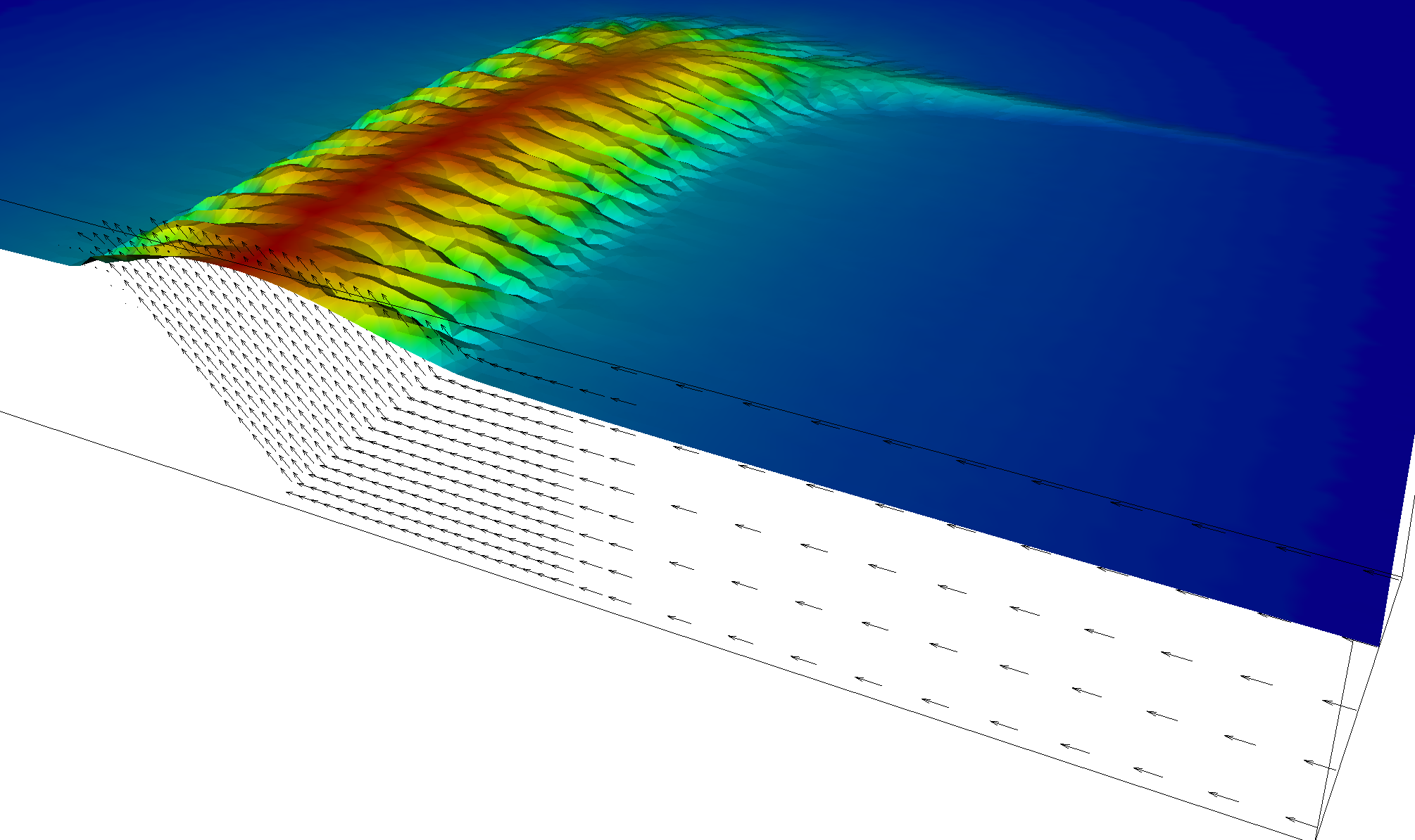
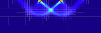
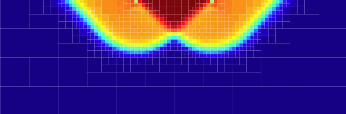
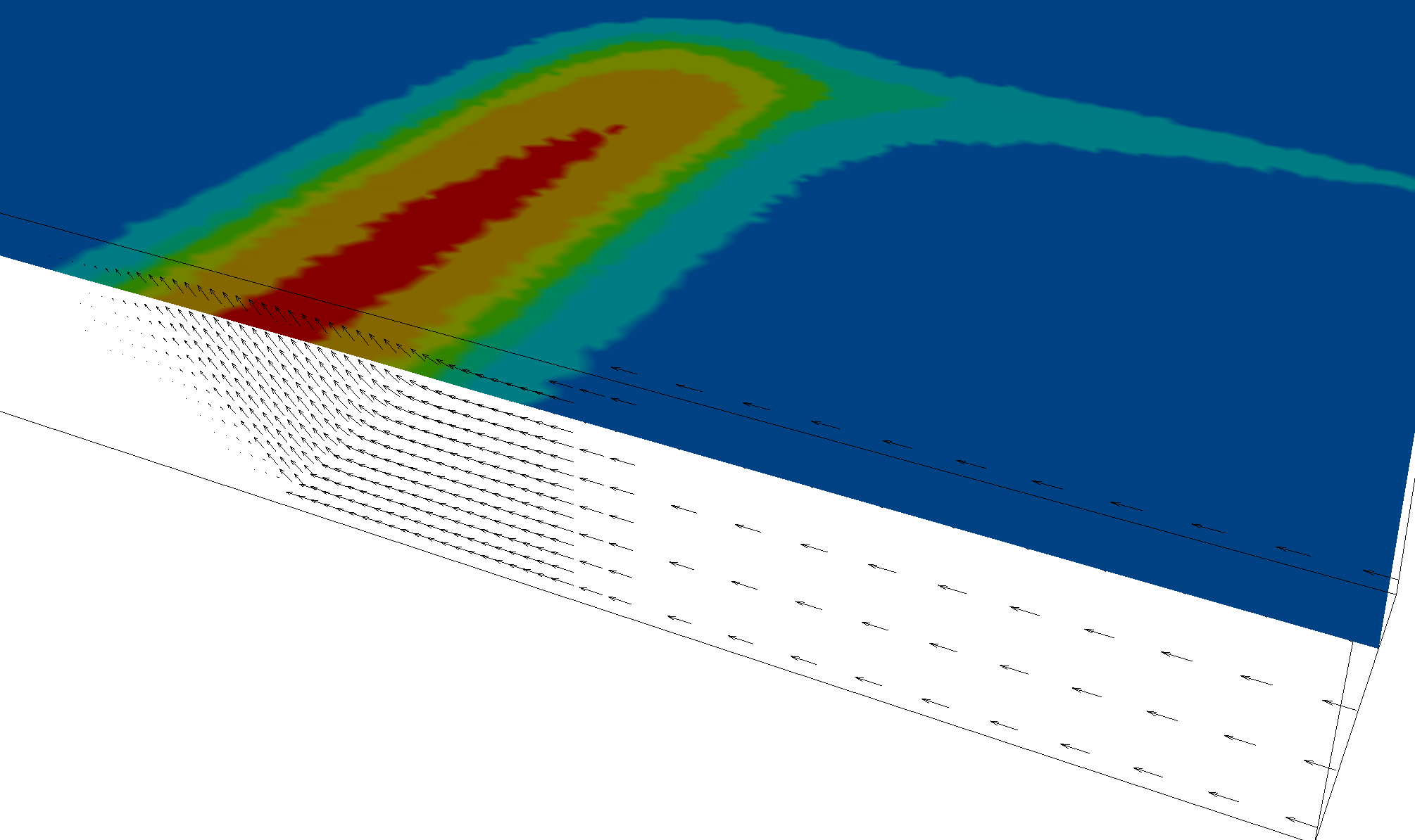
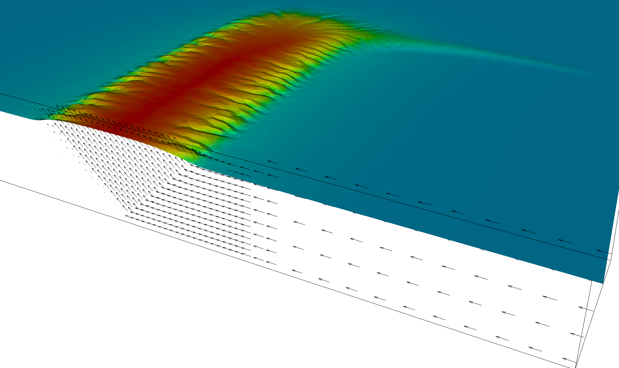
On the following figures are presented the solutions obtained on the final grid of maximum level Lmax = 8. One sees that the code has reasonnably well captured the slip-lines: the lightblue colour indicates regions where E2', the second invariant of the deviatoric strain-rate tensor, is maximal, the velocity norm shows a rigid wedge and two regions on each side of constant velocity, and the velocity field displays three regions of apparent rigid movement and two of rotation, as expected:
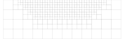
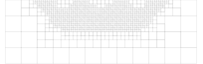
On the following figures are shown the succession of increasing level grids that were built in order to reach the final grid. Figure a) represents the portion of the initial uniform grid of interest. The solution is first computed on this grid, and is used to refine a new grid down to level 6 (Figure b). Once the solution is obtained on this grid, and as long as the refinement based on this solution leads to an octree that does not comply with the C2 criterion, the process is iterated, until we reach a stable grid (Figures c and d). It is then used to generate a level 7 grid (Figures e). After some grid iterations, the algorithm carries on to level Lmax = 8 (Figures g and h).
 b)
b)
 d)
d)
 f)
f)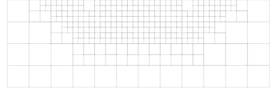
 h)
h)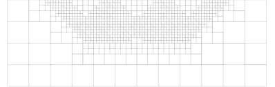
It is to be noticed that this algorithm allows for grids to evolve at a given constant level, and that, given the set of refinement parameters input by the user, it computes the best/smallest grid satisfying the conditions, hence insuring that no memory is wasted. The transition from level 7 to level 8 grids is a good illustration of this process: the refinement criterion based on the velocity field computed on grid f) overestimates the grid structure g) that ultimately evolves into h). Similar qualitative results have already been obtained previously by Zienkiewicz et al. (1995) with mainly adaptive triangular meshes.
 b)
b)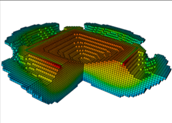
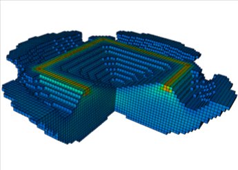
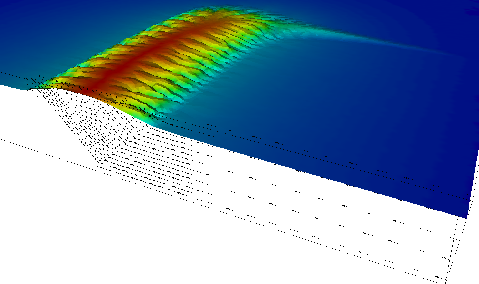
Similar experiments have already been performed in three dimensions to investigate the importance of an imposed velocity in a direction perpendicular to the shortening (folding) direction (Kaus and Schmalholz, 2006). Here, the system is further characterized by a free surface located at distance Δz = 0.05 from the top of the competent layer and subjected to very efficient erosion. Material that is eroded from the region of positive topography is deposited in the regions of negative topography simulating surface processes. An initial small perturbation in the layer thickness is imposed in the upper quarter of the model (x and y < 0.5) to force the folding to initiate near the center of the model as well as to introduce an asymmetry in the system and produce a non-cylindrical fold. The evolution of the model is shown in the following figure:
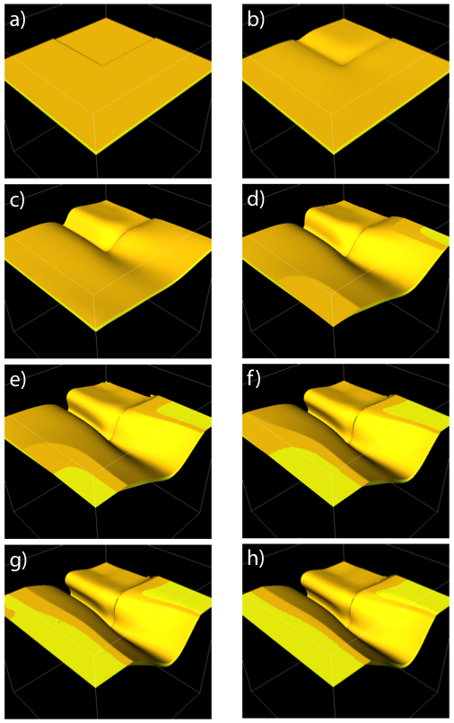
Figures a) to h) represent equally spaced time steps in the evolution of the system. The non-linear viscosity leads to the formation of a single, asymmetrical fold which rapidly grows and leads to the exhumation of the folding layer, first in the right corner of the experiment (as seen from the reader's point of view), then in the front corner. Further shortening leads to complete erosion of the folding layer along the left boundary of the model and the concomitant filling of the depression created by the down-going limb of the fold near the centre of the model. The folding instability arises from the presence of the more competent layer; as deformation progresses and the layer is exhumed, the instability stops (Figure e) and shortening is accommodated by pure shear of the entire model leading to a progressive tightening of the fold (Figure f to h).
 b)
b)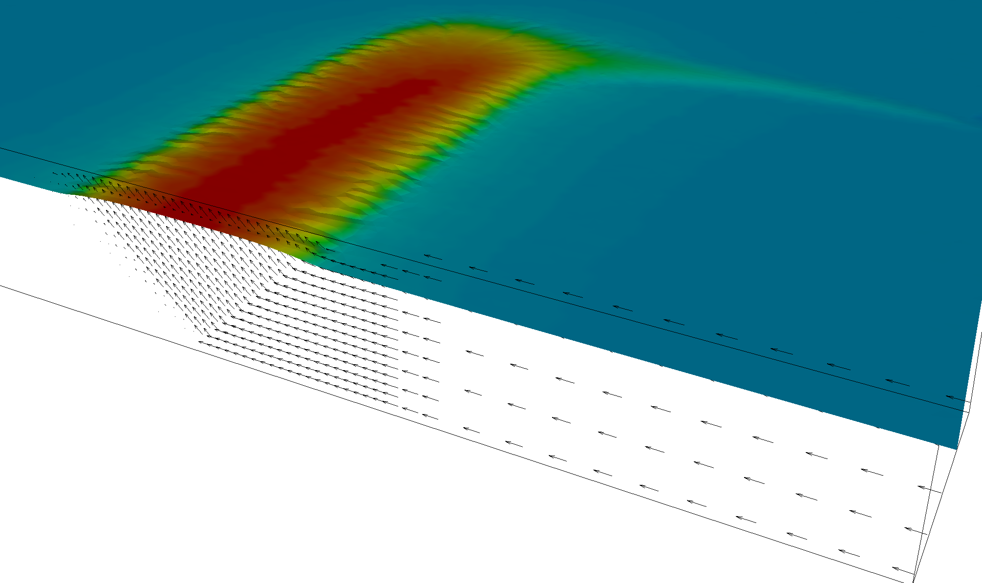
 d)
d)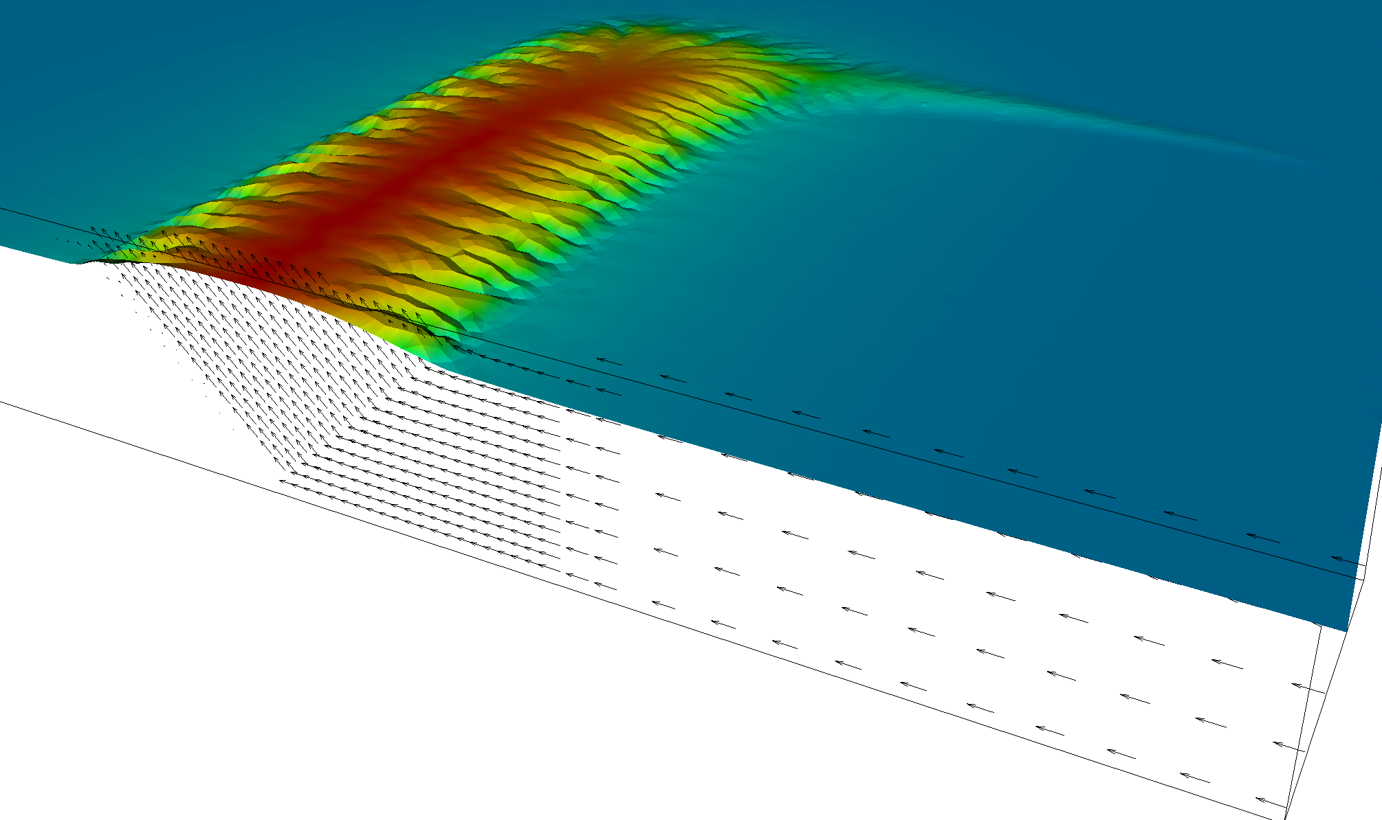
 f)
f)