SPHene is a CFD code developed in 2007. At its core is the Smoothed Particle Hydrodynamics method developped in the late 70's independently by Monaghan and Lucy. This method relies on a set of discrete points called particles that sample the fluid and carry a given mass, density, velocity, acceleration ... From these values it is possible to compute spatial gradients and higher order derivatives, such as the pressure gradient, the strain-rate or Laplacian of the velocity for every particle. In order to do so, each particle only 'sees' a given subset of its neighbours that are within a cut-off distance and attributes them a given weight by means of a kernel function.
This method is explicit in time and once the acceleration of each particle is known, it is advected and from the new spatial distribution of these particles one can compute new accelerations, and so forth.
In its standard and commonly described form, the SPH method suffers from many drawbacks, such as boundary conditions implementation, near free surface gradient estimations, conditional stability, lack of high order consistency, non unicity of derivatives discretisation, etc ... SPHene has been primarily designed as a modular code for the testing of various implementations of existing algorithms and/or new ones. This code is therefore two-dimensional only: it would be trivial to produce a three-dimensional version but memory requirements and computational time would rise up with yet no substancial benefit for the understanding of the observed phenomena. Moreover it is for the same reason sequential, even though the parallelisation of some 'bottleneck' routines would most certainly improve its performances while making it impossible to run on my old G4 laptop.
I wish to stress out that this code is currently under development and that the simulations presented on this page are by no means 'perfect'. I nonetheless show these results to later compare them to the ones obtained with improved versions of the algorithms. SPHene has been calibrated for very simple numerical experiments (Poiseuille and Couette flows for instance) only, and what follows is simply an illustration of the type of problems a purely Lagrangian code such as SPHene can tackle. It is also worth noticing that besides the specification of material properties and resolution in the input file of each of these experiments, the only necessary coding required to run them is the specification of the boundary particles and the prescribed boundary conditions, like any other CFD code.
The visualisation is based on the PGPLOT library. Convertion from postscript to png is done w ith Imagemagick, and from images to movies by means of Quicktime for the time being.
I wish to thank Mathieu Labbe for his many improvements and suggestions, the coding of the linked-list neighbour finding algorithm, the coding of the slip/no-slip boundary conditions, and for useful discussions and comments. Some figures displayed on this page come from his 3-month internship report (Spring and Fall 2007). You can download
A good starting point in the world of SPH is the book by Liu and Liu, Smoothed Particle Hydrodynamics: a meshfree particle method , at World S cientific. I must admit I do not like this book very much (structure, relevance of some topics, choice of illustrations) even though I cannot deny the wealth of information this book provides. As complementary reading, I would advise:
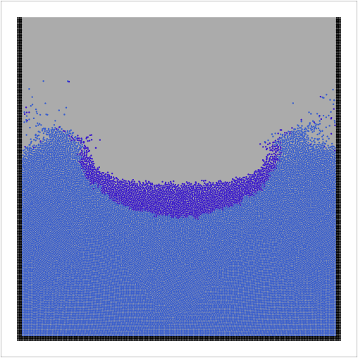
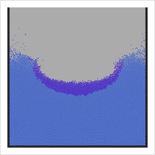
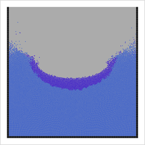
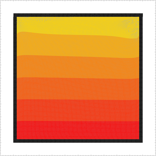
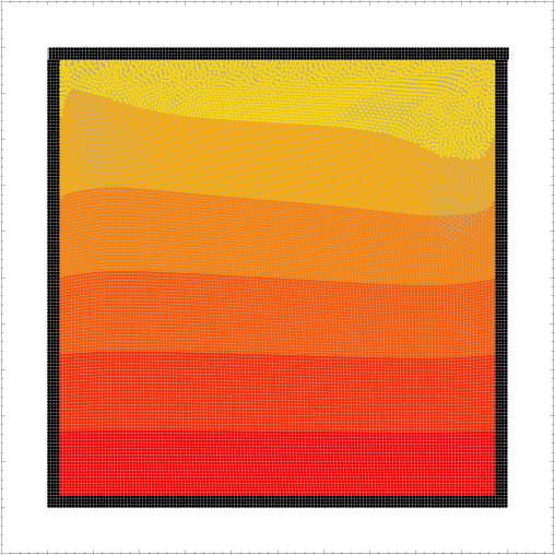
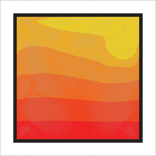
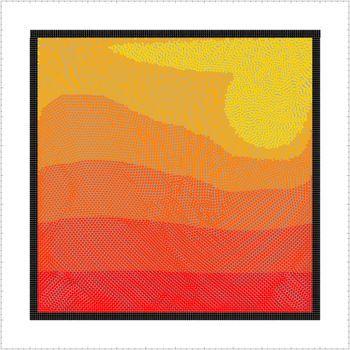
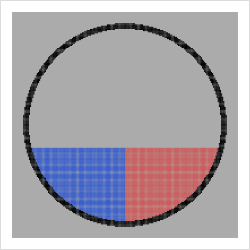
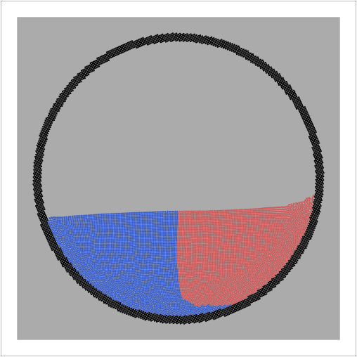
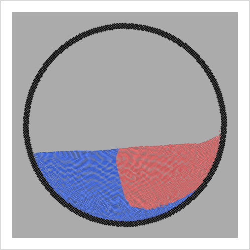
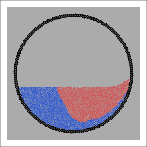
On the following snapshots a-e) of the system at different times, a row of particles was colored differently than the others from the bulk. It is then possible to observe how this line first curves as the velocity profile hasn't reached its stationary state:
a) 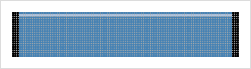 |
b) 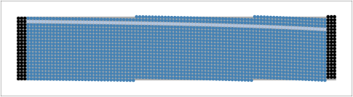 |
c) 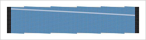 |
d) 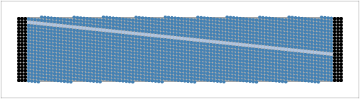 |
e) 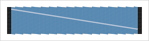 |
f) 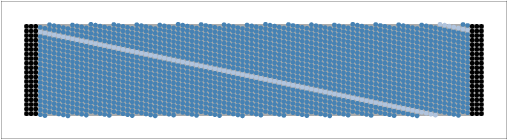 |
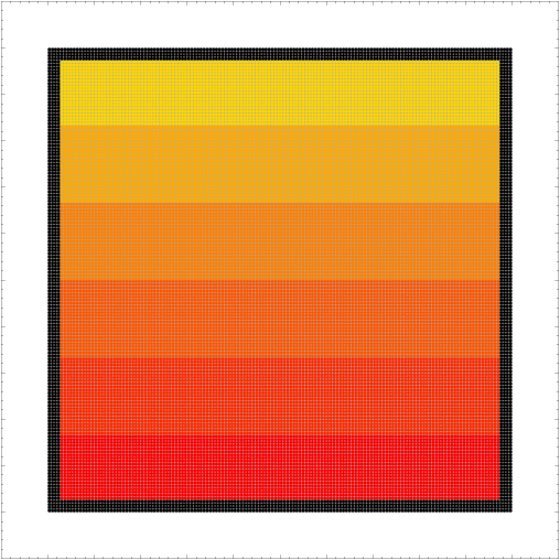
One can also colour the particles with a color scale indicating their velocity, as shown on the following a-d) plots:
a) 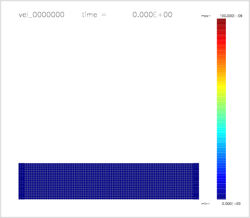 |
b) 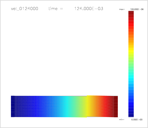 |
c) 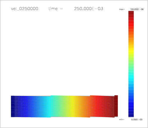 |
d) 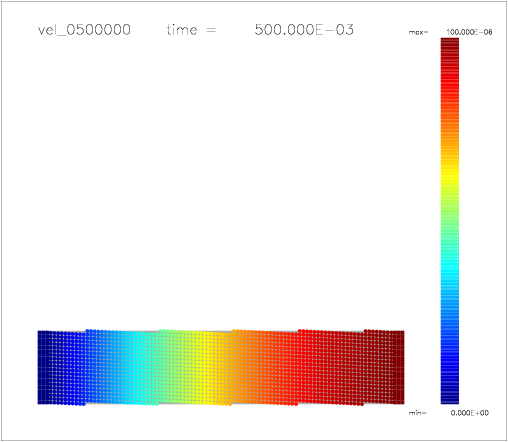 |
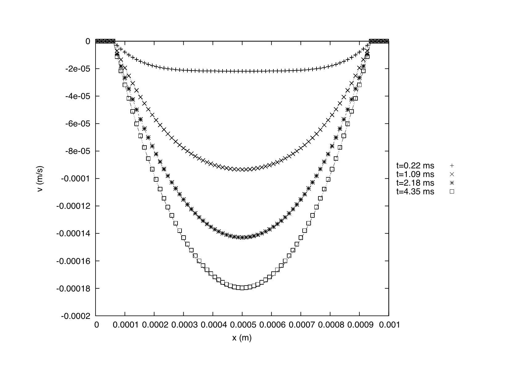
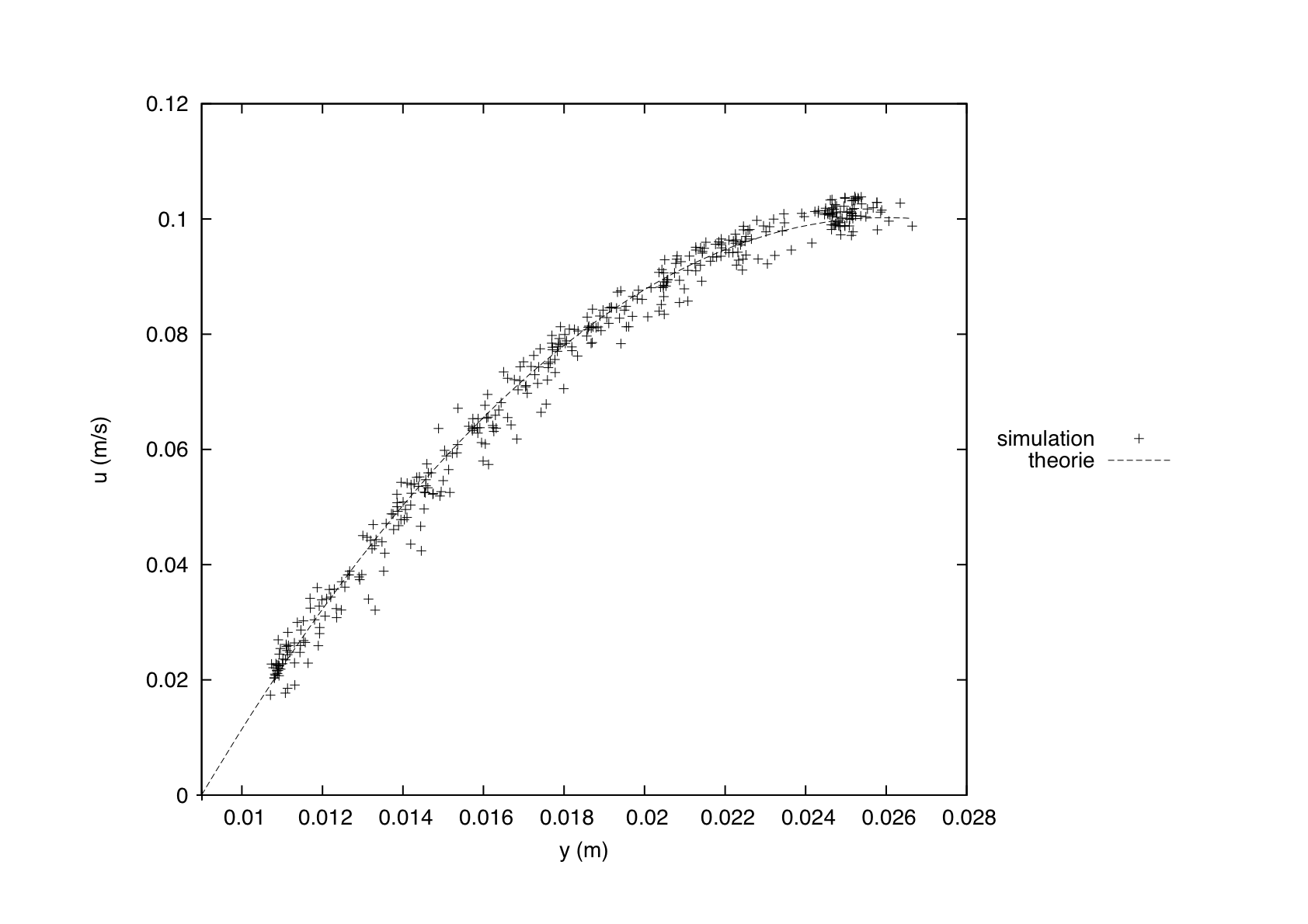
The non-stationary and stationary analytical velovity profiles are given by

so it is possible to plot on the same graph these profiles at different times, and the measured ones on the particles:
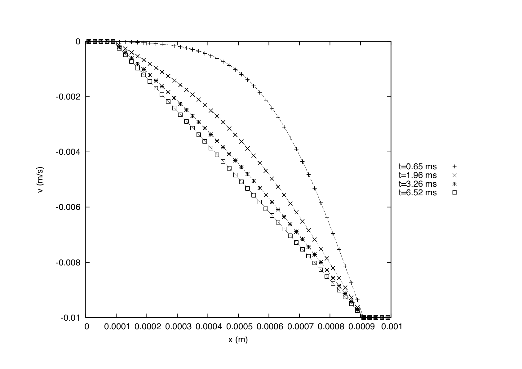
The error between the measurements and the theoretical curves is found to be less than 0.3%.
a) 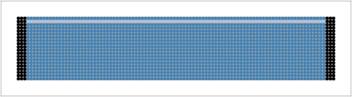 |
b) 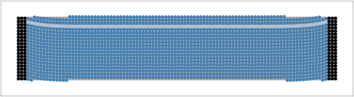 |
c) 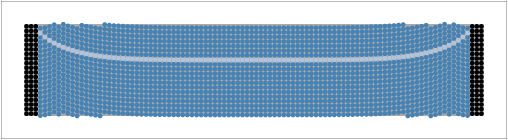 |
d) 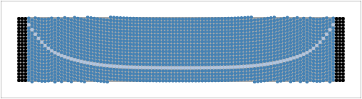 |
e) 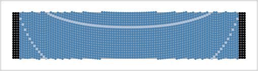 |
f) 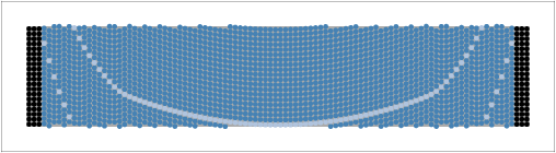 |
One can also colour the particles with a color scale indicating their velocity, as shown on the following a-d) plots:
a)  |
b) 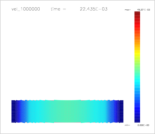 |
c) 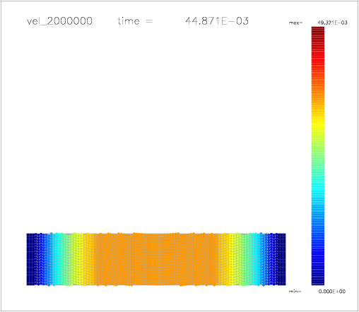 |
d) 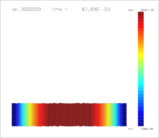 |
The non-stationary and stationary analytical velovity profiles are given by

so it is possible to plot on the same graph these profiles at different times, and the measured ones on the particles:
The error between the measurements and the theoretical curves is found to be less than 0.8%.
a)  |
b) 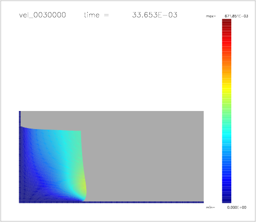 |
c) 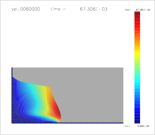 |
d) 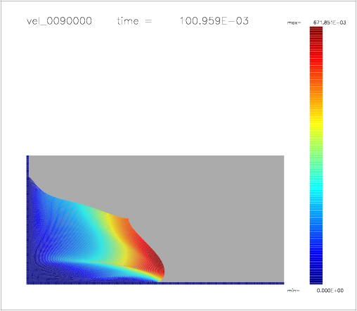 |
a) 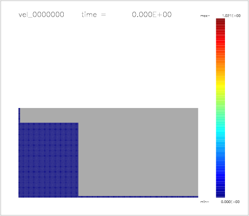 |
b) 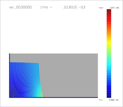 |
c) 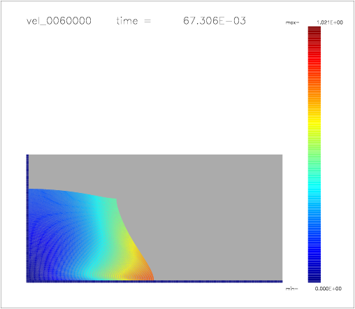 |
d) 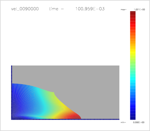 |
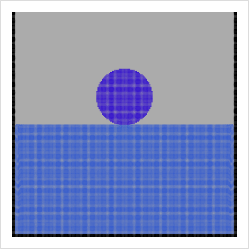
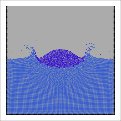
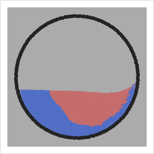
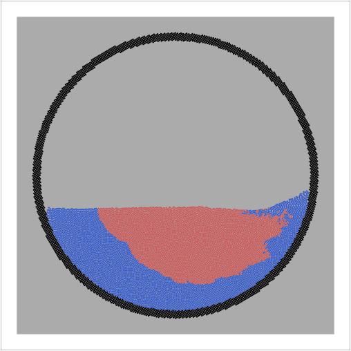
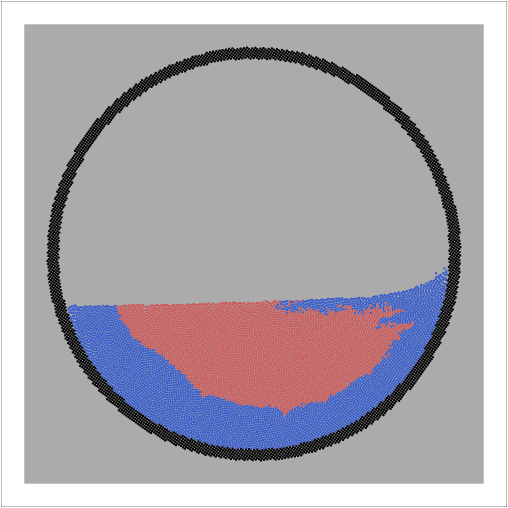
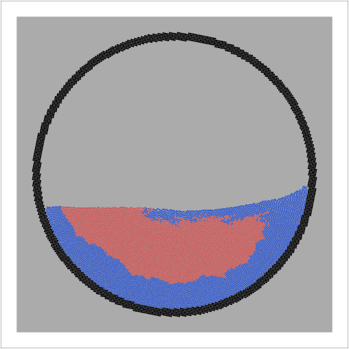
a)  |
b)  |
c)  |
d)  |
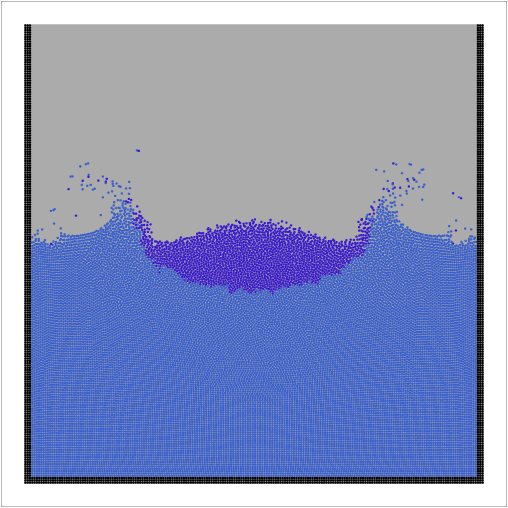
e) 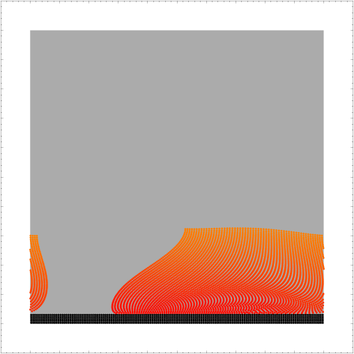 |
f) 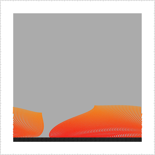 |
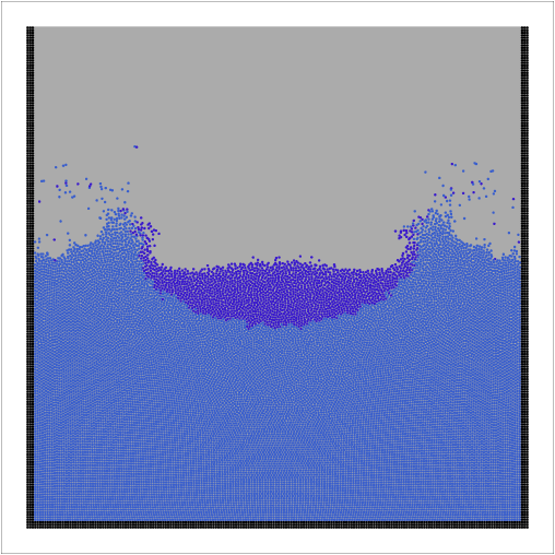
g) 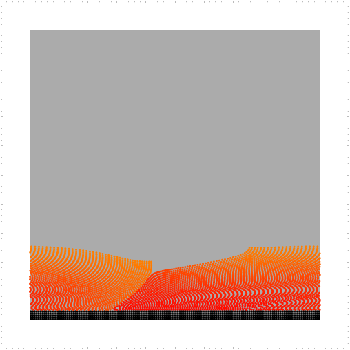 |
h) 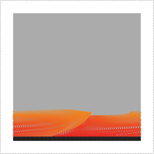 |
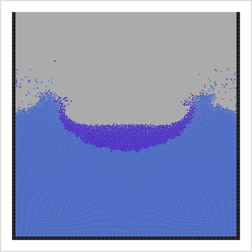
i) 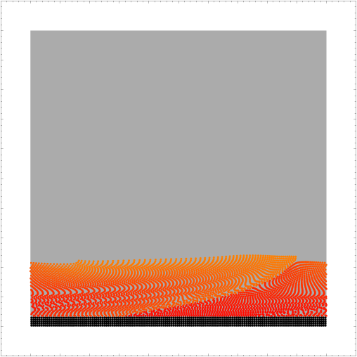 |
j) 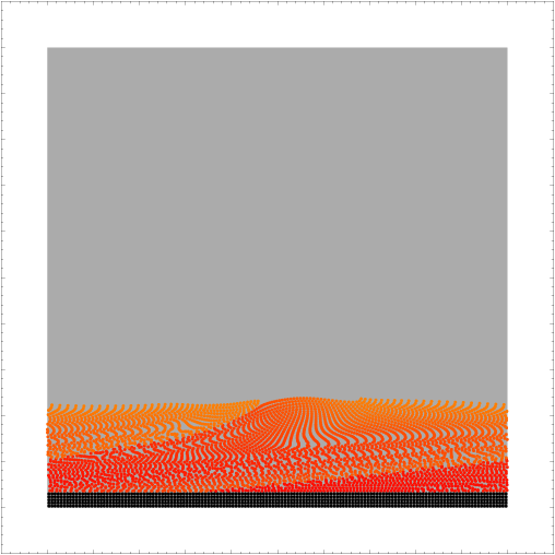 |
k) 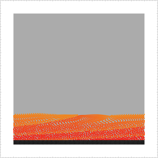 |
l) 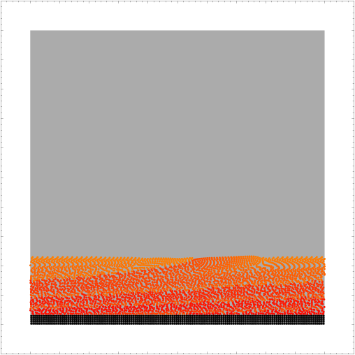 |
The expected stationary flow velocity profile is given by the following formula:
and one can plot the measured velocity profile on the SPH particle with the theoretical profile:
The dispersion error is approximately 5%.
a) 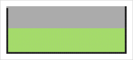 |
b) 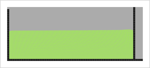 |
c) 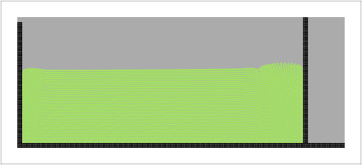 |
d) 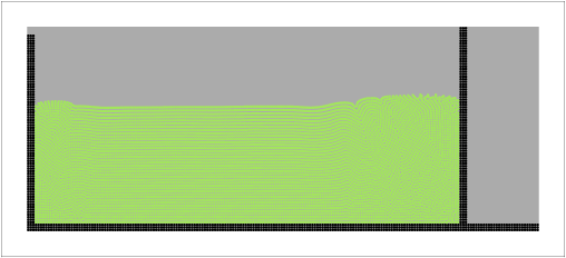 |
e) 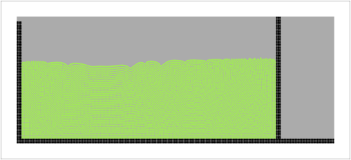 |
f) 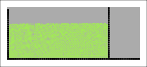 |
g) 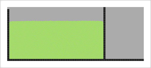 |
h) 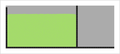 |
i) 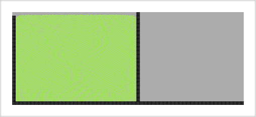 |
 |
 |
 |
 |
 |
 |
 |
 |
 |
 |
 |
 |
 |
 |
 |
 |
 |
 |
 |
 |
 |
 |
 |
 |
 |
 |
 |
 |
 |
 |
 |
 |
 |
 |
