./geodisp input.nino3
All the produced graphs will be found in the OUTPUT directory. In the following table are shown the output files:
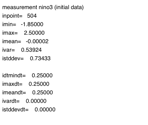 |
stats_nino3.ps inpoint is the number of data points in the nino3.dat file. imin, imean, imax, ivar, istddev are respectively the minimum, average, maximum, variance and standard deviation values of the measurements.
|
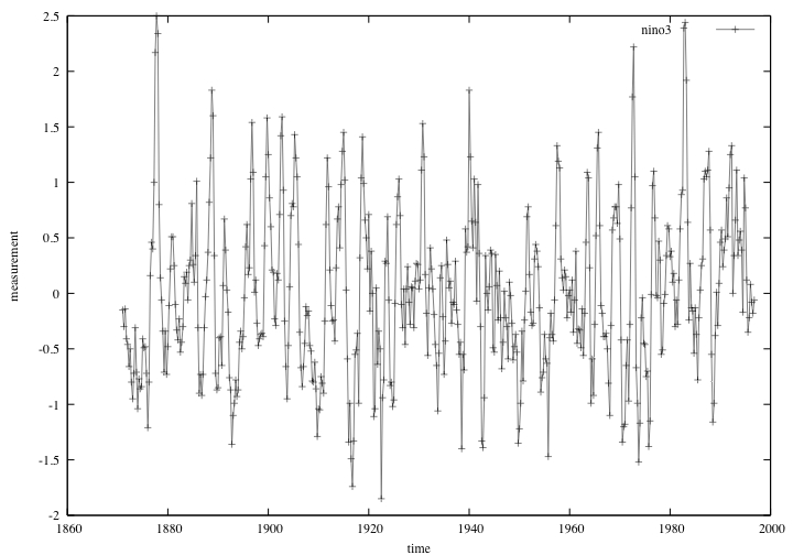 |
isignal_nino3.ps This is the actual input signal. |
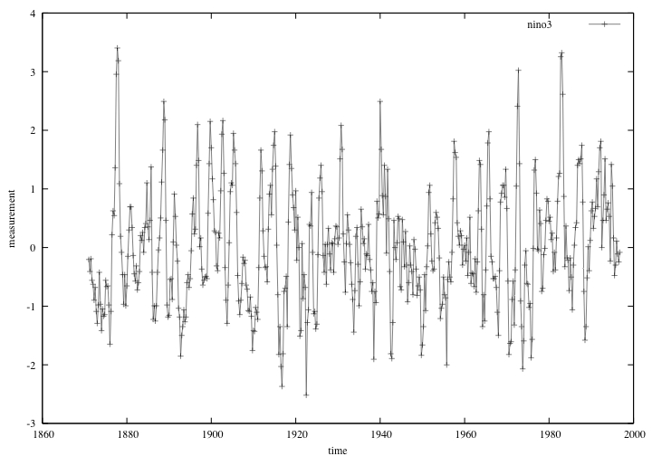 |
rsignal_nino3.ps This is the renormalised input signal. |
| |
lomb_transform_nino3.ps This represents the Lomb transform of the renormalised input signal. |
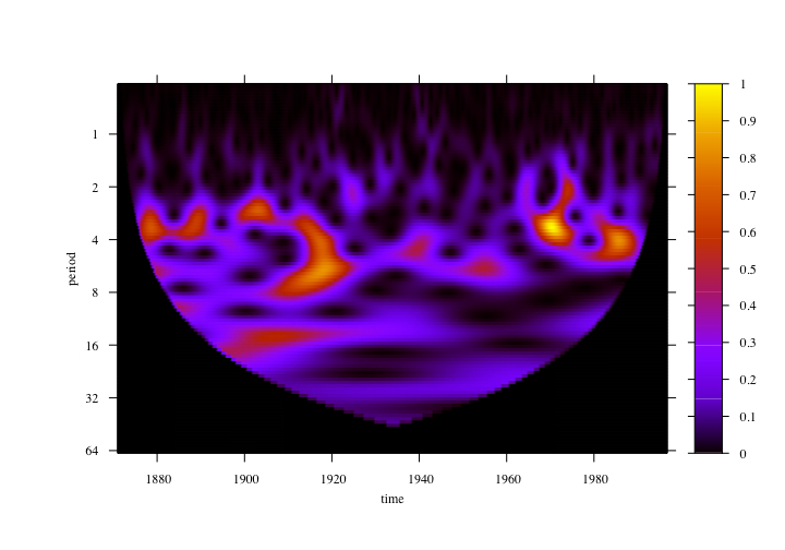 |
wave_ps_nino3.ps This represents the wavelet power spectrum of the renormalised input signal. |
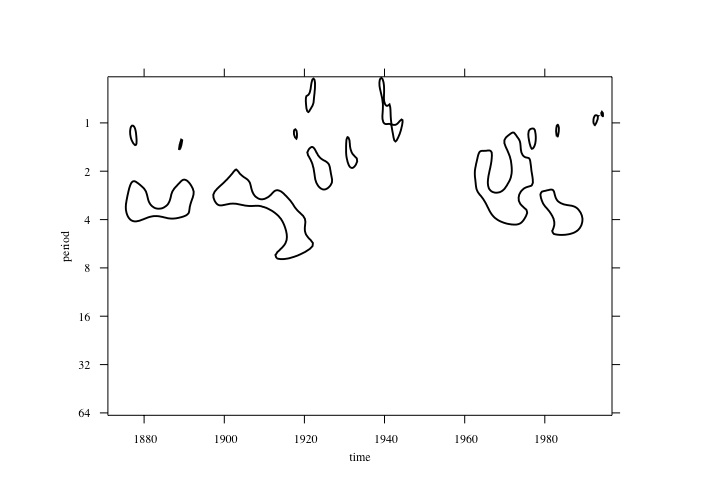 |
sig95_nino3.ps This represents the contours that enclose regions of greater than 95% confidence for a red-noise process with a lag-1 coefficient of 0.72. |
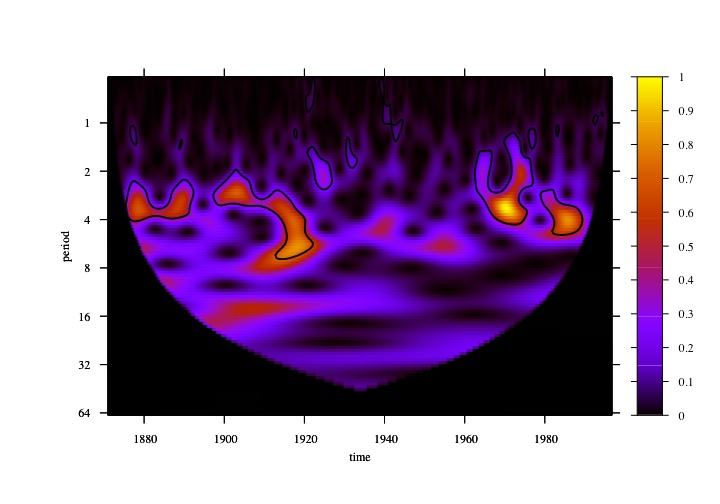 |
wave_ps_sig95_nino3.ps This represents the wavelet power spectrum of the renormalised input signal with 95% confidence contours. See Fig. 1 of Torrence and Compo. |
 |
global_ws_nino3.ps This represents the global wavelet power spectrum of the renormalised input signal. The dashed line is the 95% confidence level for the global wavelet spectrum. See Fig. 6 of Torrence and Compo. |
These last two plots are to be compared with the ones obtained by running Torrence and Compo's Matlab program on the same datafile:


Not only do the plots look alike, but output data were compared and found to match exactly within the machine precision.
